4.3 Q8: Exploring the Time Analysis by ARIMA
Building on the univariate analysis provided by LSTM in the previous section, this segment introduces VAR and ARIMA models to explore multivariate effects. These methods allow us to consider the impact of Reddit post content on Dogecoin price by incorporating multiple time series variables, thus enabling a more comprehensive analysis of how social media influences cryptocurrency markets.
4.3.1 - ARIMA(p, d, q) Model Equation
The ARIMA model combines autoregressive (AR) elements, differencing for stationarity (I), and moving average (MA) components. It is denoted as ARIMA(p, d, q), where:
- \(p\): Number of autoregressive terms
- \(d\): Number of nonseasonal differences needed for stationarity
- \(q\): Number of lagged forecast errors in the prediction equation
Differencing (I)
To achieve stationarity, the series is differenced $d $times. The differenced series \(\nabla^d y_t\) is calculated as:
\[ \nabla y_t = y_t - y_{t-1} \]
Autoregressive (AR) Part
The AR part involves using \(p\) past values:
\[ \phi_1 y_{t-1} + \phi_2 y_{t-2} + \dots + \phi_p y_{t-p} \]
Moving Average (MA) Part
The MA part incorporates the errors from \(q\) past forecasts:
\[ \theta_1 \epsilon_{t-1} + \theta_2 \epsilon_{t-2} + \dots + \theta_q \epsilon_{t-q} \]
where \(\epsilon_{t-1},\epsilon_{t-2}, \dots\) are the error terms from previous forecasts, and \(\theta_1, \theta_2, \dots, \theta_q\) are coefficients.
Combined ARIMA Equation
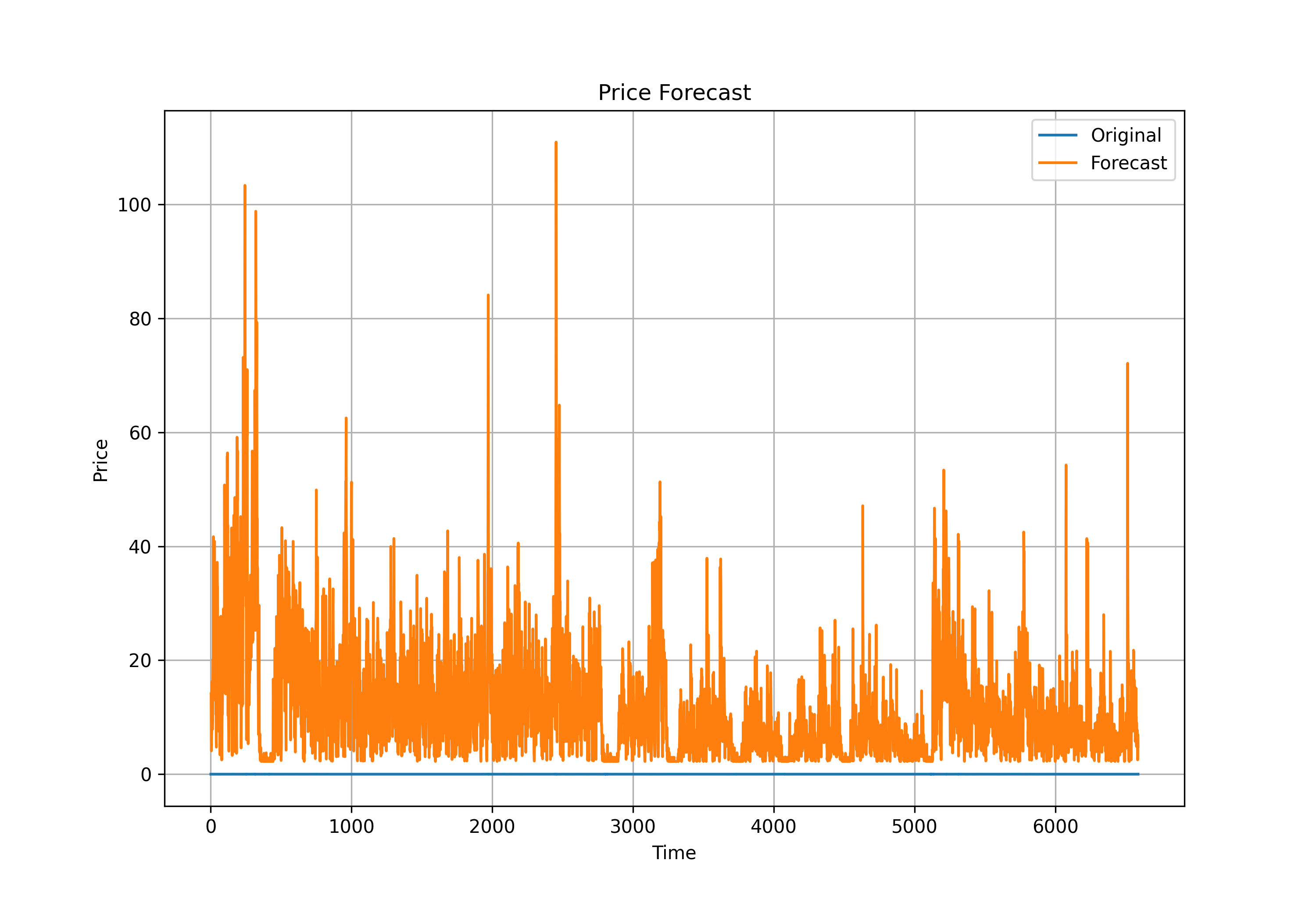
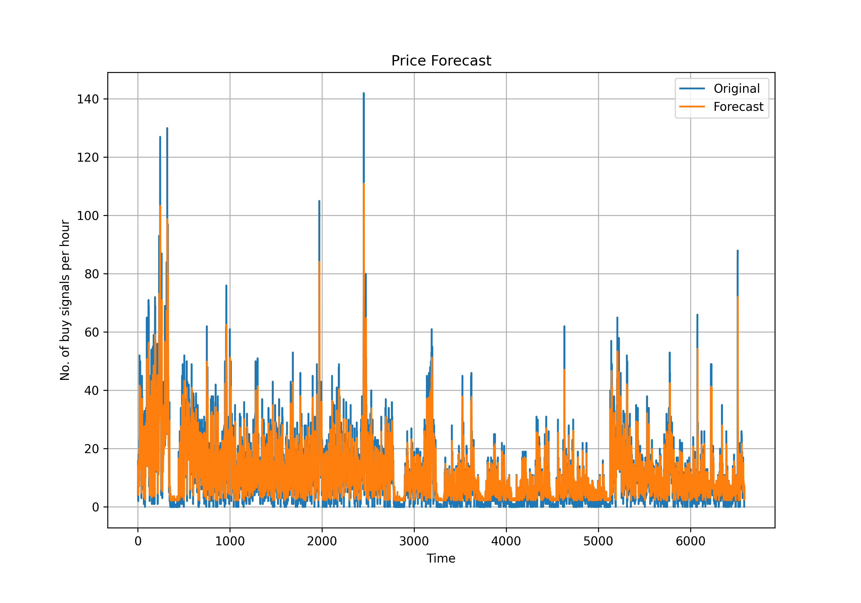
Combining these components, we run two ARIMA models with price and buy signals as dependent variables:
- Model for price (\(p=1\), \(d=1\), \(q=1\) )
\[ price_t' = c + \phi_1 price_{t-1}' + \theta_1 \epsilon_{t-1} + \epsilon_t \]
- Model for buy signals (\(p=1\), \(d=0\), \(q=1\) )
buy_signals is already stationary, so we don’t need to difference it again.
\[ buy\_signals_t = c + \phi_1 buy\_signals_{t-1} + \theta_1 \epsilon_{t-1} + \epsilon_t \]
where: - \(y_t'\) is differenced series (if \(d >0\))
Core Results of ARIMA Models
Table Summary
| Result | Dep. Variable | Observations | AIC | BIC | Log Likelihood | Const/Coef | AR.L1 | MA.L1 | Sigma^2 |
|---|---|---|---|---|---|---|---|---|---|
| Res 1 | n_buy_sig |
6586 | 45463.716 | 45490.887 | -22727.858 | 11.5079 | 0.8265 | -0.1053 | 58.2006 |
| Res 2 | price |
6586 | -67490.359 | -67469.981 | 33748.179 | NA | -0.4687 | 0.4380 | 2.07e-06 |
Interpretation of Results
Res 1 (n_buy_sig): The ARIMA(1, 0, 1) model for
n_buy_sigdemonstrates good predictability with a significant AR1 coefficient of 0.8265, suggesting a strong autoregressive term. The negative MA1 coefficient (-0.1053) indicates a slight adjustment in the opposite direction of the error term from the previous period. The model has a relatively high AIC and BIC, pointing to the complexity of the model but a necessary fit for the data characteristics.Res 2 (price): For the
pricevariable modeled with ARIMA(1, 1, 1), the coefficients for both AR1 and MA1 are significant but with opposite signs, suggesting partial offsetting effects. The model achieves an extremely low AIC and BIC, indicating an excellent fit. The Log Likelihood is exceptionally high, which, combined with a very low sigma^2, points to a highly effective model for forecastingprice.


4.3.2 Vector Autoregression (VAR)
Vector Autoregression (VAR) is a statistical model used to capture the linear interdependencies among multiple time series. VAR models generalize the ARIMA model by allowing more than one evolving variable. Each variable in a VAR model is a linear function of past lags of itself and past lags of the other variables. This makes VAR suitable for systems where the variables influence each other.
A VAR model describes each variable with an equation that combines:
- The variable’s own lags (autoregressive part).
- The lags of other variables in the system.
To illustrate the standard form of a VAR model for variables $y_t $ and $x_t $, the equations for this system can be expressed as:
\[ \begin{align*} y_t &= c_1 + \phi_{11} y_{t-1} + \phi_{12} x_{t-1} + \epsilon_{1t} \\ x_t &= c_2 + \phi_{21} y_{t-1} + \phi_{22} x_{t-1} + \epsilon_{2t} \end{align*} \]
Wh \(c_1\) and \(c_2\) are constants (intercepts of the equations).
\(\phi_{11}\), \(\phi_{12}\),\(\phi_{21}\), and \(\phi_{22}\) are the coefficients of the lagged values of \(y\) and \(\epsilon_{1t}\) and \(\epsilon_{2t}\) $are the error terms, assumed to be white noise.
Condensed Summary of VAR Model Results
| Equation | Lag | Coefficient | Std. Error | t-stat | Prob |
|---|---|---|---|---|---|
| price_s | |||||
| L1.price_s | -0.027636 | 0.012353 | -2.237 | 0.025 | |
| L2.price_s | 0.031450 | 0.012355 | 2.546 | 0.011 | |
| L7.price_s | 0.041803 | 0.012343 | 3.387 | 0.001 | |
| L9.price_s | 0.033151 | 0.012362 | 2.682 | 0.007 | |
| L11.price_s | -0.025686 | 0.012359 | -2.078 | 0.038 | |
| n_buy_sig | |||||
| L1.n_buy_sig | 0.707021 | 0.012347 | 57.265 | 0.000 | |
| L2.price_s | -136.544667 | 64.626404 | -2.113 | 0.035 | |
| L4.n_buy_sig | 0.068851 | 0.015113 | 4.556 | 0.000 | |
| L7.price_s | 178.560081 | 64.568315 | 2.765 | 0.006 | |
| L10.n_buy_sig | 0.034079 | 0.015100 | 2.257 | 0.024 | |
| L11.n_buy_sig | 0.036609 | 0.012330 | 2.969 | 0.003 |
Equation for price_s
\[ price_{s,t} = -0.027636 \cdot price_{s,t-1} + 0.031450 \cdot price_{s,t-2} + 0.041803 \cdot price_{s,t-7} + 0.033151 \cdot price_{s,t-9} - 0.025686 \cdot price_{s,t-11} + \epsilon_{t} \]
Equation for n_buy_sig
\[ n\_buy\_sig_t = 0.707021 \cdot n\_buy\_sig_{t-1} - 136.544667 \cdot price_{s,t-2} + 0.068851 \cdot n\_buy\_sig_{t-4} + 178.560081 \cdot price_{s,t-7} + 0.034079 \cdot n\_buy\_sig_{t-10} + 0.036609 \cdot n\_buy\_sig_{t-11} + \epsilon_{t} \]
Impulse response functions (IRF)
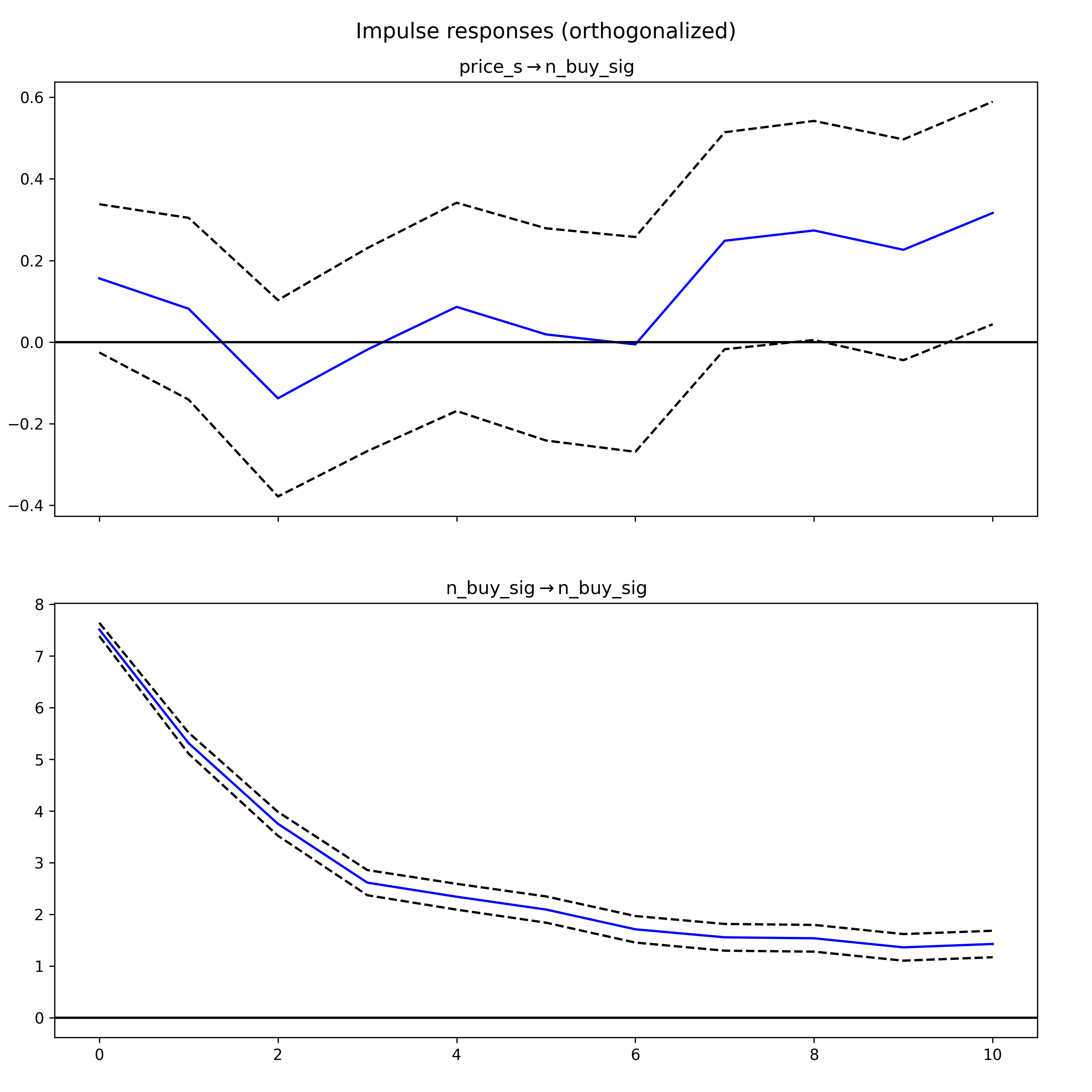
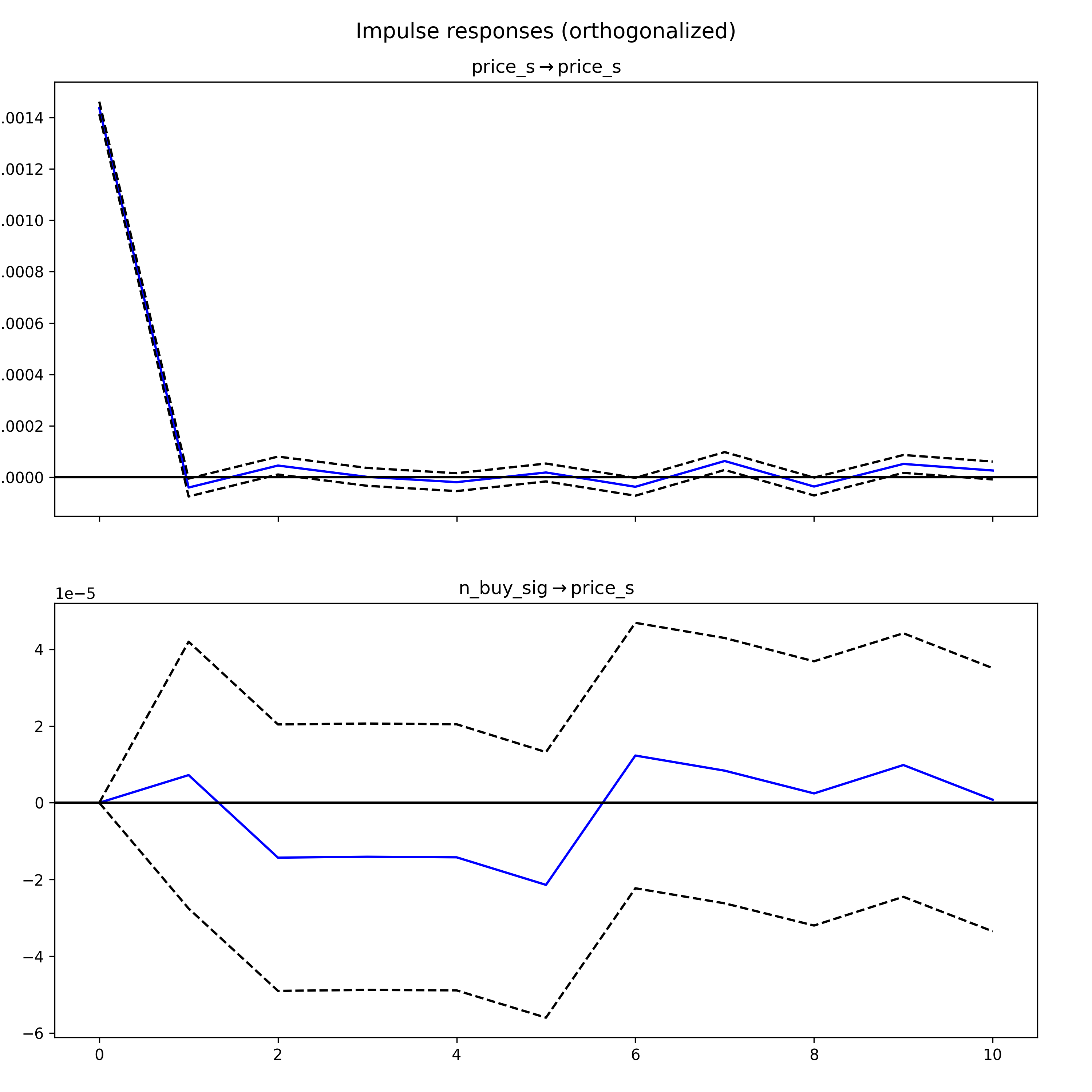
In Vector Autoregression (VAR) models, an IRF maps the reaction of endogenous variables in the model to a one-unit increase in the shock variable, holding all else constant. In the following IRF chart, the response of price_s (differenced price for stationarity) to a shock in n_buy_sig is displayed over several hours.
The components of an IRF plot are explained below:
- X Axis: Displays the time intervals following a shock (hours)
- Y Axis: Measures the magnitude of the response from the dependent variable ($for price, number of buy signals)
- Blue Line: Represents the estimated response of the variable to the shock across different time periods.
- Dashed Lines: These indicate the confidence intervals, showing the range where the true response likely falls, typically with a 95% confidence level.
A response line that crosses the zero line signifies changes in the direction of the response over time.
(If the confidence interval includes the zero line, it indicates that the response is not statistically significant at those points.)
In the first IRF graph, the response of “price_s” to shocks in “n_buy_sig” is observed. Initially, the response drops below zero, indicating a negative impact, before oscillating around zero. This pattern suggests an immediate negative reaction followed by ongoing uncertainty in both the direction and magnitude of the impact.
The second IRF graph examines the response of “n_buy_sig” to shocks in “price_s.” The response begins at zero, then dips into the negative territory and exhibits a pattern of oscillation that gradually returns toward zero. The diminishing amplitude of the response over time suggests that the impact of the shock lessens as time progresses.


